Topological sorting is about ordering objects that are initially only partially ordered. This issue is relevant to many problems discussed in introductory OR/MS textbooks, yet for some unexplained reason most textbooks do not tell their readers how this task can be accomplished. Presumebaly it is assumed that for the small problems discussed in textbooks students are able to figure out how to do this "by inspection". In this paper we take a more formal look at this task and provide an online interactive module for experimentation with simple topological sorting tasks. We call on OR/MS courseware developers to re-examine their position with regard to this topic.
Here is how the algorithm works:
The next candidate node to be processed can be any node satisfying the following two conditions: (a) It has not yet been re-labeled and (b) it does not have any active immediate predecessor.
When a node is processed, two things happen: first, the next label is assigned to it and second, all the arcs emanating from this node are deactivated.
The algorithm terminates when none of the nodes satisfies these conditions. If this is because all the nodes have been re-labeled, then the problem is acyclic and the new labels are in increasing order. If the algorithm terminates because each of the unlabeled nodes has at least one active immediate predecessor then the problem is cyclic: each of the unlabeled nodes is involved in a cycle with one or more of the other unlabeled nodes.
We now apply this algorithm to the problem represented by the following graph. We shall replace the given labels A,B, ..., G by 1,2,...,7.
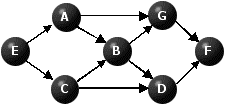
Figure 1
There is one node that has not been re-labeled yet having no immediate predecessors, namely E. We re-label it, 1, and deactivate the arcs emanating from it.
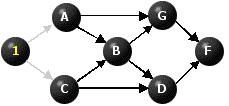
Figure 2
There are now two no nodes with no immediate predecessors that have not yer been relabeled, namely A and C. We select one of them, say A, label it 2 and deactivate the arcs emanating from it.
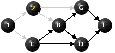
Figure 3
There is now one node with no immediate predecessors that has not yet been relabeled, namely C. We label it 3 and deactivate the arcs emanating from it.
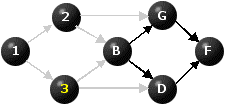
Figure 4
There is now one node with no immediate predecessors, that has not yet been relabeled, namely B. We label it 4 and deactivate the arcs emanating from it.
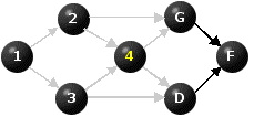
Figure 5
There are now two nodes with no immediate predecessors that have not yet been relabeled, namely G and D. We select one of them, say G, label it 5 and deactivate the arcs emanating from it.
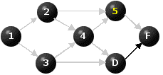
Figure 6
There is now one node with no immediate predecessors that has not yet been re-labeled, namely C. We label it 6 and deactivate the arcs emanating from it.
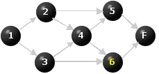
Figure 7
There is now one node with no immediate predecessors that has not yet been re-labeled, namely C. We label it 7.
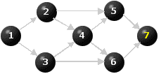
Figure 8
All the nodes have been re-labeled, so we stop. The graph is acyclic.
In contrast, consider the following cyclic graph.
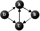
Figure 9
There is one node with no immediate predecessors, namely D. We label it 1 and deactivate the arcs emanating from it.
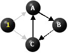
Figure 10
There are no nodes with no immediate predecessors that have not yet been re-labeled. So we stop. Since not all the nodes have been relabeled, we conclude that the subgraph consisting of the remaining nodes is cyclic.
Needless to say, for large problems it is not convenient to use the graphic approach. Instead, we can use binary incident matrices to describe graphs. In such a matrix row i represents the immediate successors of node i and column j represents the immediate predecessors of node j. Here we use black cells to represent "Yes" in these matrices. At the bottom of the matrix we list the total number of active immediate predecessors of each column (T(j)) and the new label allocated to it (L(j)). The following sequence of incident matrices describes the re-labeling procedure.
 Figure 1 |
|
There is one column j such that T(j) = 0 and j has not yet been re-labelled, namely j = E. So we set L(E)=1 and dim the black cells in row E.
 Figure 2 |
|
There are now two columns j such that T(j) = 0 and j has not yet been re-labelled, namely j = A and j = C. So we set L(A)=2 and dim the black cells in row A.
 Figure 3 |
|
 Figure 4 |
|
 Figure 5 |
|
 Figure 6 |
|
 Figure 7 |
|
 Figure 8 |
|
You can use the module below to experiment with the algorithm. To specify the incident matrix click the relevant cells of the matrix. When ready, click the Algorithm radio button. To relabel a node click the respective red square in the C row. The algorithm terminates when there are no red squares.

 You might be interested in using a more elaborate module that will enable you to
- solve much large problems
- control the size of the graph
- generate pseudo-random problems
- use pre-set examples
This module also offers a more elaborate on-line help services.